
Modeling and simulation of vertical roller mill using population balance model
Download Article in PDF format
Rasoul Fatahi, Kianoush Baran
Department of Mining Engineering, Lorestan University, Khorramabad, Iran
Corresponding author: barani.k@lu.ac.ir (Kianoush Barani)
Abstract: There are few studies concerning the process simulation of vertical roller mills (VRMs). In this research work, the application of population balance model for simulation of a VRM in a cement clinker grinding circuit was investigated. The residence time distribution (RTD) was measured, and the tank-in-series and Weller models were employed to describe the residence time distribution. Two sampling surveys were carried out on the VRM circuit. The data from the first survey were used for model calibration, and the specific breakage rates were back-calculated. The model parameters obtained were used for simulation of the second survey, and validation of the model. The results showed that the clinker particle spent a short time inside the VRM and the mean residence time is about 67s. The tanks-in series model compares to Weller model was more proper to describe the residence time distributions in the VRM. The simulation results showed that the specific breakage rates increased with increasing particle size. However, the particles larger than 25.4 mm particles sizes are too large to be properly nipped by master rollers. Finally, it can be concluded that the grinding process of the VRM is very well-predictable with the population balance model.
Keywords:vertical roller mill, modeling, simulation, cement grinding, residence time distribution
1. Introduction
Grinding operation is one of the important parts of the cement production processes. Almost producing one ton of cement requires 1.5 tons of raw materials. The electrical energy consumed in the cement production process is approximately 110kWh/ton, about 30% of which is used for the preparation of the raw materials and about 40% for clinker grinding (Jankovic et al., 2004).
The grinding energy consumption in a cement plant is a major issue which most of this energy is wasted as heat and noise. The application of vertical roller mills (VRMs) for ore grinding is a part of the strategies against rising energy consumption (Reichert et al., 2015).
The VRM technology was introduced in the mid-’90s for grinding clinker and slag by LOESCHE (Schaefer, 2001). Fig. 1 illustrates the grinding parts of a Loesche vertical roller mill.
The grinding material is comminuted in the Loesche roller grinding mill between the rotating horizontal grinding track and stationary grinding rollers. Grinding is affected primarily by compression. A certain amount of shear force increases the number of fine particles in the grinding material. This effect is created by tapered rollers, whose axes are angled at 15˚ with respect to the horizontal grinding track. Hot gas is supplied to the combined drying and grinding process to evaporate material moisture. In the classifier above the grinding chamber, the finished material is separated from the grit, which can drop back onto the grinding table to be comminuted again
(Schafer, 2003).
The VRMs have advantages compare to conventional grinding technology. In the VRMs, the particles are ground in a particle bed; the bed breakage is more energy-efficient and usually produces a narrower particle size distribution (Fuerstenau, 1992; Viljoen et al., 2001). The breakage predomi-
DOI: 10.5277/ppmp19064
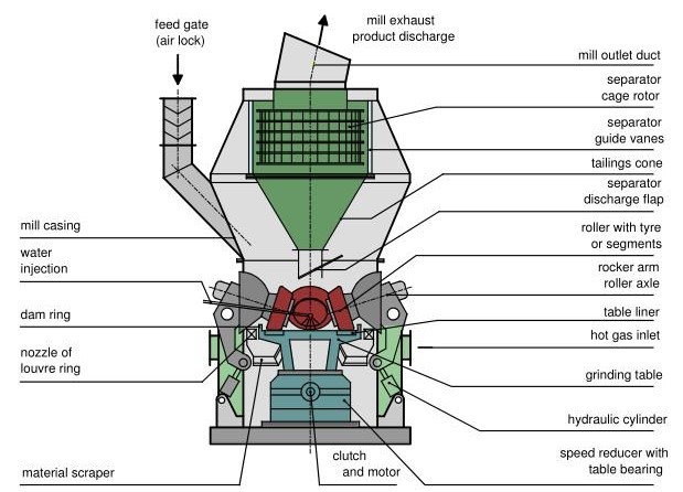
Fig. 1. Schematic operation principle of a vertical-roller-mill
nantly occurs by particle-particle-contacts or phase–phase-contacts(Fandrich et al., 2007). Both breakage modes enhance the liberation of the valuable mineral phases, which may lead to further improvements in the beneficiation process (Reichert et al., 2015). Also, Due to a dry grinding process, no process water is required, which will become more critical in the next decades. VRM’s are widely used in the coal and cement industry today (Reichert et al., 2015). However, a disadvantage of VRMs is the vibration of the rolls that is caused by the frictional characteristics (Fujita and Saito, 2006).
Simulation is the best way to optimize a grinding circuit to achieve economical operation. There are few studies on the simulation of VRMs.
The matrix model was used to simulated vertical roller mills in cement clinker and coal grinding lines. The pressure breakage function, B, was determined from the laboratory test data with a hammer device. The results showed that materials are crushed in more than one stage under the vertical roller mill. However, in the paper, it is unclear that the selection functions, S values, was obtained from the test data, back-calculation ,or literature (Wang et al., 2009).
The matrix model was used for simulation of a VRM with high-efficiency slat classifier in OMYA’s limestone processing plant in Eger, Hungary, on a technology with Pfeiffer’s 2800 C vertical roller grinding mill. The B breakage matrices were simply determined by the well-known Broadbent-Calcott function. A systematic test was carried out to grind the limestone samples in a laboratory Hardgrove mill to verify this assumption. The selection matrix, S, and the number of breaking stages, v, were determined by the iterative computer simulation processing using the measured data(Faitli et al., 2014).
Optimization, modeling, and simulation of VRM in a cement raw mix grinding circuit with the perfect mixing ball mill model were studied. A series of samplings were conducted around the raw mix grinding circuit, and clinker samples were taken. The data obtained from the plant sampling was fitted with the perfect mixing ball mill model using the steady-state mineral processing software, the JKSimmet. The breakage function and the breakage rate function for VRM were determined during the model fitting process. The Broadbent and Callcott equation was used as the breakage function. It was found that raw mix grinding in a VRM could be described by the perfect mixing model. In a perfect mixing ball mill, the feed entering the mill would be distributed along with the mill, thus being subjected to the probability for breakage. A similar situation was encountered in a VRM, where the feed that had fallen on the grinding table was being subjected to the breakage process by the rollers, and the entire particles would have some probabilities for breakage (Palaniandy et al., 2006).
Application of the perfect mixing model for simulation of a VRM in a cement clinker grinding plant was investigated. The breakage distribution function of the material was determined by the compressed bed breakage test in a piston-die cell device. The model parameters were back-calculated using the feed and product size distribution data and the breakage distribution function. The simulation results showed that the simulated product size distribution curve fitted the measured product curve quite well (Shahgholi et al., 2017).
In the industrial grinding processes, the output particle size strongly depends on the mill residence time. The residence time distribution (RTD) must be measured to evaluate mill performance and identify breakage rates. In none of the previous studies, the RTD in simulation has not been considered. Almost no work has been done to measurement and modeling of residence time distribution of VRMs. RTD estimation in a VRM is complex due to different components in the mill, the mass transport characteristics, and solid segregation. In the present research, we have done a survey to determine mill RTD to understand the mixing regime better, and simulate the VRM with population balance model.
2. Materials and methods
2.1. Surveying and sampling
This study was performed in Ilam cement plant. Ilam cement plant is located in Ilam province, west Iran. The plant has two cement production lines and totally produces 5300 t/day cement. In this study, the second production line was surveyed. The cement raw materials (lime, silica and iron ore) enter the circuit through two apron feeders. The raw materials are crushed in a hammer crusher to D95 of 80mm. The raw materials are mixed in a certain proportion and fed into a vertical roller mill (LOESCHE mill). The vertical roller mill grinds the marital to D85 of 90µm. The ground product is calcined in a preheater to 850-900℃. After calcination, the materials enter to a rotary kiln and heated to 1450℃ to become clinker. The clinkers are cooled by six fans and entered the clinker bins. The D90 of clinkers are 32mm. The clinkers and gypsum with a ratio of 97 to 3% are interred to a vertical roller mill (LOESCHE mill). The feed rate of the clinker VRM is 160t/h. The VRM has four rollers including two big rollers (master rollers) and two small rollers (slave roller), which respectively perform grinding and make material layering on the grinding table. Fig. 2 shows the simplified flow sheet of the VRM grinding circuit at Ilam cement plant.
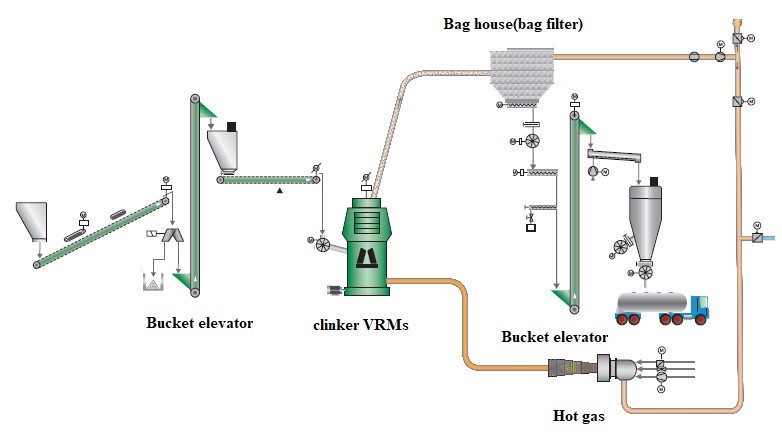
Fig. 2. The VRM grinding circuit at Ilam cement plant
Two surveys were carried out on the grinding circuit. The data collected from the first survey (feed and product) was used for modeling and simulation of the circuit, and the second survey was used for validation of the model parameters. For any survey, samples weighing 100 kg were collected from the conveyor feed belt and the mill product for two hours with 10 minutes interval. The mill outlet is a channel that the ground product sucked at high speed by an air separator. Sampling from this channel was a challenging task. For this purpose, a sampler was designed and manufactured (Fig. 3). The sampler was a steel tube with a length of 1.2m (The width of the channel) and a diameter of 50mm. A hole was embedded in the channel. There was a slot at the end of the tube where the particles trapped and fall into the end due to the gravity. The sample of feed was riffled and sized by screening and also the sample of the product analyzed by laser particle size analyzer.
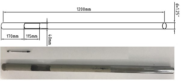
Fig. 3. The designed and manufactured sampler
2.2. RTD measurement
The RTD was measured by carrying out an impulse test using zinc concentrate powder (zinc sulfide) (35% Zn) as a tracer. Zinc sulfide powder was chosen for this purpose because there is no zinc in cement raw materials, and zinc can be analyzed by a traditional analytical method such as AAS and ICP. The powder was mixed with cement, some water, and pelletized. The tracer was carefully prepared so that its size distribution was similar to the size distribution of the clinker in the feed of the VRM. The weight of tracer impulse was calculated in such a way that after dilution and mixing with the mil content is measurable at the VRM product. 100 Kg of the pellets was suddenly injected in the feed stream entering the mill. Approximately every 10-20 seconds the sampler enters the mill outlet channel for two seconds and one sample was taken. The samples were analyzed for zinc by using atomic absorption spectrometry (Agilent, 240FS AA model).
If the tracer is injected as a pulse, then the fraction of tracer that remains in the mill at any time (assuming constant flow rate through the mill) can be defined by the distribution function E(t) mathematically as follows (Makokha et al., 2011):
E (() (1)
where C(t) is the tracer concentration in the outlet stream as a function of time and C(t)dt defines the area under the curve.
The first and second moment of the RTD function around the origin gives the mean residence time (MRT or 𝜏01) and the variance (𝜎3) (𝑤𝑖𝑑𝑡ℎ 𝑜𝑓 𝑡𝑟𝑎𝑐𝑒𝑟 𝑐𝑢𝑟𝑣𝑒3) respectively, where the latter is a measure of the spread of the RTD curves about the mean value.
𝑀𝑅𝑇 . dt (2)
. dt (3)
The MRT represents the mass transfer phenomenon, which equals to the vessel volume to volumetric feed rate, and the variance refers to the degree of mixing which occurs within the vessel. It is particularly useful for fitting experimental curves to the theoretical curves.
In this research, the tanks-in-series and Weller models were evaluated. The models were applied to obtained experimental data to evaluate their applicability. Parameters of every model were optimized by minimizing the squared error between experimental tracer response data and model predictions. Data analysis and modeling were carried out using the solver tool in the Excel spreadsheet.
Weller model proposes a different approach representing the mill mixing regime as several perfectly mixed reactors in series either with equal or different sizes. This model allows the mill behavior to be described by a condition between a plug-flow and a perfect mixing regime. It comprised one large perfect mixer (τL) and two small perfect mixers in series (τS), including a dead time or plug- flow regime (τPF) (Eq. 4):
E(t) = KJL [− NOKKRPQ exp (− NOKKVPQ) − α exp X− NOKKVPQY + α exp X− NOKKLPQY] (4)
where a = tL/(tL – tS).
The tanks-in-series model is a good model to describe turbulent flow in pipes, laminar flow in very long tubes, flow in packed beds, shaft kilns, long channels, screw conveyors, etc. The tanks-in-series model is simple, can be used with any kinetics, and it can be extended without too much difficulty to any arrangement of compartments, with or without recycle (Levenspiel, 1962). Eq. (5) describes the tanks-in-series model mathematically:
E(t) = \](^)]f]_(‘\abcOg )(!_]e(d)) (5)
where n is number of tanks and τ is means residence time.
2.3. Breakage distribution function
The breakage function used in this study was obtained from our previous study data (Shahgholi et al., 2017). In our previous study, the breakage function was determined by the well-explored lab-scale compressed bed breakage test in a piston-die cell device. The data were fitted by Eq. (6)(Austin et al., 1984).
𝐵j,g = 𝜑(mm‘n )o + (1 − 𝜑)(mm‘n )q (6)
where xi and x1 are the size of friction i th and the first fraction respectively, and φ, γ and β are model parameters, and R is relative size (x/x)ratio of i-th and first size fraction. By fitting the Eq. (6) to the previous data the model parameters were calculated (φ = 0.966, γ = 0.31863 and β=0.31862).
2.4. Population balance model
For the modeling of continuous steady-state mills, the breakage equation is combined with the material residence time distribution. The two extremes of residence time distributions are plug flow and fully mixed. For plug flow, all materials have the same residence time, and hence the batch grinding equation is applicable when integrated from time zero to the residence time. The solution to this integration was originally proposed by Reid (Reid, 1965) and is known as the Reid solution.
The general form of the solution is:
𝑚j(𝑡) = ∑jtug 𝑎jt 𝑒vw^ 𝑓𝑜𝑟 𝑁 ≥ 𝑖 ≥ 1 (7)
where
⎧ 0 𝑖 < 𝑗 ⎪ 𝑚j(0) − ∑jOugg 𝑎j 𝑖 = 𝑗
𝑎jt = j g (8)
⎨⎪⎩ vnOvw jOugt 𝑆 𝑏j 𝑎t 𝑖 > 𝑗
For i > 2 the number of terms in the expression expands rapidly.
For a fully mixed mill at steady state, the equation becomes
𝑃j jtOugg 𝑏jt 𝑆t𝑚t − 𝑆j𝑚j𝜏 𝑓𝑜𝑟 𝑁 ≥ 𝑖 ≥ 𝑗 ≥ 1 (9)
j g
n ∑nw_‘‘ nwvw f w
𝑃j = g vnf (10)
where τ = mean residence time.
According to Eq. (10), to measuring the size distribution of product the mill (𝑃j), mean residence time (τ), selection functions of different classes (𝑆j), breakage functions (𝑏jt), and mass in the screen classes (𝑚j) must be determined.
By placing, 𝑏jt, 𝐹j and 𝑃t in the Eq. (10) for the 𝑆t values can be back-calculated in the Excel
spreadsheet environment or Matlab.
3. Results and discussion
3.1. RTD measurement
Fig. 4 illustrates the deviation of experimental data from the estimated values using tanks-in-series model Weller models. The shape of obtained RTD curves depends on the combined effect of the flow behavior and mixing performance inside the mill, which was usually related to the RTD function parameters, i.e., MRT and variance. Table 1 presents the statistical parameters of RTD models for the experimental data. As seen the R2 of the tanks-in- series model was higher than that by Weller model, and also the relative variance (𝑅10 j0\ = ) resulted from the tanks-in- series model was lower than that by Weller model. In other words, it can be stated that the tanks-in- series model is more suitable for experimental data compared to Weller model then the tanks-in-series model was used for modeling of mixing regime and estimate the means residence time.
The results showed that the clinker particle spent a short time inside the VRM, and the mean residence time is about 67s. The short time residence time shows that the number of breakages for particles in the VRM is one to three times, which avoids any unnecessary over-grinding.
The long tail in this curve is a result of the recycling of tracer, and presence of stagnant volume with exchange or both. The fine particles maybe after 2-3 times breakage are sucked by air separator and exited the VRM. Coarse particles are too large to be properly nipped by master rollers then they are forced to the edge of the table and fallen to the circulate stream or moved to the stagnant regions.
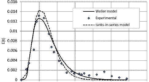
Fig. 4. Fitting the tank-in- series and Weller models to th practical data at feed rate 160t/h
Table 1. Statistical components of the tanks-in-series and Weller RTD models
| Model | Term | value |
| Weller | τpf(s) τl(s) τs(s)
Means residence time (s) |
10.597 31.504 16.445
74.991 |
| R square | 0.925 |
Relative variance 0.273
Means residence time (s)
| tanks-in-series | N
R square |
5
0.955 |
| Relative variance | 0.2 |
3.2. Model calibration
Fig. 5 shows the measured particle size distribution of the VRM feed and product. The Rosin-Rammler particle size distribution function was fitted to the feed and product size distribution from Fig. 2, and the mathematical feed and product size distributions for 28 size classes were calculated (column 3 and 4 in Table 2). The non-cumulative breakage function was calculated from Eq. (6) (φ = 0.96582, γ = 0.31863 and β=0.31862) (column 5 in Table 2). From Eq. (10) (τ=67s) the selection function values (Si) were back-calculated (column6 in Table 2).

Fig. 5. Measured particle size distribution of feed and product of the VRM
Fig. 6 shows specific breakage rates (S values) plotted against particle size. It can be seen that the maximum breakage rate is at the particle size of 25.4 mm. The specific breakage rate of the particles size of 31.75 mm is to the right of maximum in the curve; it means the particles sizes are too large to be properly nipped by master rollers then they are forced to the edge of the table and fall to the circulate stream or move to the stagnant regions. The specific rate of breakage was decreased with decreasing the particle size from 25.4 mm to zero so that the specific rate of breakage of particles under 100µm is about zero. Particles with a size smaller than 100µm have no chance to be ground, and even agglomeration may occur.
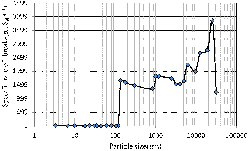
Fig. 6. Variation of specific rates of breakage versus particle size
Table 2. Model fitting results
1 31750 8.25 0 0 1231.328 2 25400 25.25 0 0.069 3853.603
3 19050 16.05 0 0.081 2761.144 4 12700 13.6 0 0.103 2659.323 5 9525 7.35 0 0.072 1989.723
- 6300 25 0 0.077 2240.694
- 5000 45 0 0.042 1651.842 8 4000 2.8 0 0.038 1531.031
9 3150 2.7 0 0.037 1529.194 10 2500 4.2 0 0.034 1742.121 11 1190 4.03 0 0.093 1827.032
12 1000 2.77 0 0.019 1819.301 13 841 0.1 0 0.018 1366.591 14 297 0.38 0 0.088 1484.855
15 177 0.01 0 0.034 1593.665 16 138.038 0.61 0 0.014 1663.084
17 120.33 0.03 1.02 0.008 0.134 18 104.71 0.02 0.7 0.007 0.189
- 43 0.04 2.52 0.013 0.042
- 26 0.03 4.64 0.012 0.015
- 71 0.02 7.25 0.011 0.003
- 67 0.01 9.61 0.01 -0.002
- 2 0.01 5.4 0.005 0.005
- 91 0.01 11.13 0.009 -0.006
- 38 0.01 10.56 0.008 -0.007 26 10 0.01 16.7 0.014 -0.011 27 6.607 0.01 8.89 0.009 -0.009
28 3.311 0 9.56 0.013 -0.011
3.3. Validation of model
Sampling data from the second survey was used for validation of the model parameters. The grinding condition such as the feed rate, operating pressure, and other mill setting parameters was the same as the first survey. Thus, it was assumed that the S values were not changed. Fig. 7 shows the simulation results. It could be seen that the size distribution of the simulated product fitted well on the measured product (coefficient of determination or R-squared = 0.99), and the population balance model gave a right prediction. The result of this work compared to our previous work (Shahgholi et al., 2017) shows that population balance model compared with perfect mixing model gives a better prediction for simulation of the VRMs in cement grinding processes.
4. Conclusions
In this study, the residence time distribution of a vertical roller mill in a cement clinker grinding circuit was experimentally measured using zinc powder as a tracer. It was revealed that the tank-in-
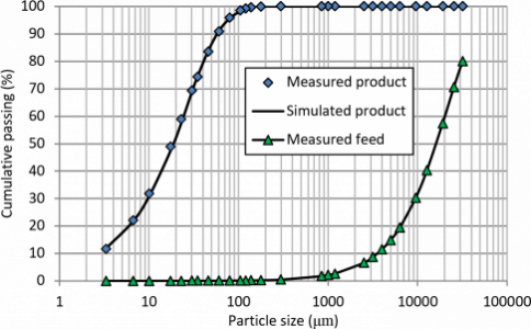
Fig. 7. Comparison between simulated and measured product size distributions
series model is appropriate to describe the residence time distributions in the VRM. The results showed that the clinker particle spent a short time inside the VRM, and the mean residence time is about 67s. The short time residence time shows that the number of breakages for particles in the VRMs is one to three times, which avoids any unnecessary over-grinding. The RTD curve has a long tail that can be due to the recycling of the tracer, the presence of stagnant volume with exchange or both.
The population balance model was used for modeling of the VRM vertical upon the survey data. The results showed that the specific breakage rates increased with increasing particle size. However, the particles larger than 25.4 mm is too large to be adequately nipped by master rollers. The simulation results showed that the simulated product size distribution curves fit the measured product curves quite well. It can be concluded that the grinding process of a VRM is very wellpredictable with the population balance model.
However, for the proper use of the population balance model for VRM simulation, further research works with different feed in different plants are required.
Acknowledgments
The authors would like to thank the management and all staff of Ilam Cement Plant for their sincere co-operation during plant visits and sampling campaigns
References
AUSTIN, L.G., KLIMPEL, R.R., LUCKIE, P.T., 1984. Process Engineering of Size Reduction: Ball Milling, AIME, SME, NewYork, USA. SME-AIME New York, USA.
FAITLI, J., CZEL, P., 2014. Matrix Model Simulation of a Vertical Roller Mill with High-Efficiency Slat Classifierr. Chemical Engineering & Technology 37, 779–786.
FANDRICH, R., GU, Y., BURROWS, D., MOELLER, K., 2007. Modern SEM-based mineral liberation analysis. Int. J. Miner. Process 84, 310–320.
FUERSTENAU, D.W., 1992. Comminution: past developments, current innovation and future challenges, in: Proceedings of the International Conference on Extractive Metallurgy of Gold and Base Metals. pp. 15–21.
FUJITA, K., SAITO, T., 2006. Unstable vibration of roller mills. Journal of sound and vibration 297, 329–350.
JANKOVIC, A., VALERY, W., DAVIS, E., 2004. Cement grinding optimisation. Minerals Engineering 17, 1075–1081.
LEVENSPIEL, O., 1962. Chemical reaction engineering, 3rd ed. John Wiley & Sons.
MAKOKHA, A.B., MOYS, M.H., BWALYA, M.M., 2011. Modeling the RTD of an industrial overflow ball mill as a function of load volume and slurry concentration. Minerals Engineering 24, 335–340.
PALANIANDY, S., AZIZLI, M., AZIZI, M.D.K., 2006. Optimization, Modeling And Simulation Of Vertical Roller Mill In Cement Raw Mix Grinding Circuit. Universiti Sains Malaysia.
REICHERT, M., GEROLD, C., FREDRIKSSON, A., ADOLFSSON, G., LIEBERWIRTH, H., 2015. Research of iron ore grinding in a vertical-roller-mill. Minerais Engineering 73, 109–115.
REID, K.J., 1965. A solution to the batch grinding equation. Chemical Engineering Science 20, 953–963.
SCHAEFER, H.U., 2001. Loesche vertical roller mills for the comminution of ores and minerals. Minerals Engineering 14, 1155–1160.
SCHAEFER, H.U., 2003. Loesche mills for the cement industry. ZKG INTERNATIONAL 56, 58–64.
SHAHGHOLI, H., BARANI, K., YAGHOBI, M., 2017. Application of perfect mixing model for simulation of vertical roller mills. Journal of Mining and Environment 8, 545–553.
VILJOEN, R.M., SMIT, J.T., DU PLESSIS, I., SER, V., 2001. The development and application of in-bed compression breakage principles. Minerals Engineering 14, 465–471.
WANG, J.-H., CHEN, Q.-R., KUANG, Y., LYNCH, A.J., ZHUO, J., 2009. Grinding process within vertical roller mills:
experiment and simulation. Mining Science and Technology (China) 19, 97–101.